My holiday reading on modularity has led me into some of the literature on the evolution of complexity. Some of the most interesting work in theoretical biology that I've read in a while relates to the ideas of nearly neutral networks and holey adaptive landscapes, an area developed by Sergey Gavrilets at the University of Tennessee. The various papers of his to which I refer can be accessed on his website. I find his explanations very clear, but recognize that this work is fairly technical stuff and my understanding of it is greatly facilitated by previous experience with similar models in the context of epidemics on networks (believe it or not). Nonetheless, a reasonably accessible introduction can be found in his 2003 chapter, "Evolution and speciation in a hyperspace: the roles of neutrality, selection, mutation and random drift." I have based much of my discussion here on this paper along with his 1997 paper in JTB.
The father of American population genetics and Modern Evolutionary Synthesis pioneer Sewall Wright first came up with the metaphor of the adaptive landscape in 1932. The basic idea is a kind of topographic map where the map coordinates are given by the genotype and the heights above these coordinates are given by the fitnesses associated with particular genotype combinations. A landscape, of course, is a three dimensional object. It has a length, a width (or latitude and longitude) and height. This particular dimensionality turns out to be very important for this story.
A major concern that arises from the idea of an adaptive landscape is how populations get from one peak to another. In order to do this, they need to pass through a valley of low fitness and this runs rather counter to our intuitions of the way natural selection works. The usual way around this apparent paradox is to postulate that populations are small and that random genetic drift (which will be more severely felt in small populations) moves the population away from its optimal point on the landscape. Once perturbed down into a valley by random forces, there is the possibility that the population can climb some other adaptive peak.
This is a slightly unsatisfying explanation though. Say that we have a finite population of a diploid organism characterized by a single diallelic locus. Finite populations are subject to random drift. The size of the population is  . Assume that the fitnesses are
  ,
,  , and
, and  . This is actually a very simple one-dimensional adaptive landscape with peaks at the ends of the segment and a valley in between. Assume that the resident population is all
  . What happens to a mutant
  allele? We know from population genetics theory that the probability that a completely neutral (i.e.,
  ) mutant allele reaching fixation is
  . Russ Lande has shown that when the
  this probability becomes:
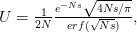
where  is the error function
  .
.
When  (say a population size of 200 and a fitness penalty of
  ), this probability is approximately
  . So for quite modest population size and fitness disadvantage for the heterozygote, the probability that the population will drift from to
  is very small. This would seem to spell trouble for the adaptive landscape model.
Gavrilets solved this conundrum -- that moving between peaks on the adaptive landscape appears to require the repeated traversing of very low-probability events -- apparently by thinking a little harder about the Wrightean metaphor than the rest of us. Our brains can visualize things very well in three dimensions. Above that, we lose that ability. Despite all the Punnett squares we may have done in high school biology, real genotypes, of course, are not 2 or 3 dimensional. Instead, even the simplest organism has a genotype space defined by thousands of dimensions. What does a thousand dimensional landscape look like? I haven't the faintest idea and I seriously doubt anyone else does either. Really, all our intuitions about the geometry of such spaces very rapidly disappear when we go beyond three dimensions.
Using percolation theory from condensed matter physics, Gavrilets reveals a highly counter-intuitive feature of such spaces' topology. In particular, there are paths through this space that are very nearly neutral with respect to fitness. This path is what is termed a "nearly neutral network." This means that a population can drift around genotype space moving closer to particular configurations (of different fitness) while nonetheless maintaining the same fitness. It seems that the apparent problem of getting from one fitness peak to another in the adaptive landscape is actually an artifact of using low-dimensional models. In high-dimensional space, it turns out there are short-cuts between fitness peaks. Fitness wormholes? Maybe.
Gavrilets and Gravner (1997) provide an example of a nearly neutral network with a very simple example motivated by Dobzhansky (1937). This model makes it easier to imagine what they mean by nearly neutral networks in more realistic genotype spaces.
Assume that fitness takes on one of two binary values: viable and non-viable. This assumption turns our space into a particularly easy type of structure with which to work (and it turns out, it is easy to relax this assumption). Say that we have a three diallelic loci ( ,
,  , and
, and  ). Say also that we have reproductively isolated "species" whenever there is a difference of two homozygous loci -- i.e., in order to be a species a genotype must differ from the others by at least homozygous loci. The reproductive isolation that defines these species is enforced by the fact that individuals heterozygous at more than one locus are non-viable. While it may be a little hard to think of this as a "landscape", it is. The species nodes on the cube are the peaks of the landscape. The valleys that separate them are the non-viable nodes on the cube face. Our model for this is a cube depicted in this figure.

Now using only the visible faces of our projected cube, I highlight the different species in blue.

The cool thing about this landscape is that there are actually ridges that connect our peaks and it is along these ridges that evolution can proceed without us needing to postulate special conditions like small population size, etc. The paths between species are represented by the purple nodes of the cube. All the nodes that remain black are non-viable so that an evolutionary sequence leading from one species to another can not pass through them. We can see that there is a modest path that leads from one species to another -- i.e., from peak to peak of the fitness landscape. Note that we can not traverse the faces (representing heterozygotes for two loci) but have to stick to edges of the cube -- the ridges of our fitness landscape. There are 27 nodes on our cube and it turns out that 11 of them are viable (though the figure only shows the ones visible in our 2d projection of the cube).
So much for a three-dimensional genotype space. This is where the percolation theory comes in. Gavrilets and Gravner (1997) show that as we increase the dimensionality, the probability that we get a large path connecting different genotypes with identical fitness increases. Say that the assignment of fitness associated with a genotype is random with probability  that the genotype is viable and
  that it is non-viable. When is small, it means that the environment is particularly harsh and that very few genotype combinations are going to be viable. In general, we expect to be small since most random genotype combinations will be non-viable. Percolation theory shows that there are essentially two regimes in our space. When
  , where
  is a critical threshold probability, the system is subcritical and we will have many small paths in the space. When
  , we achieve criticality and a giant component forms, making a large viable evolutionary path traversing many different genotypes in the space. These super-critical landscapes are what Gavrilets calls "holey". Returning to our three dimensional cube, imagine that it is a chunk of Swiss cheese. If we were to slice a face off, there would be connected parts (i.e., the cheese) and holes. If we were, say, ants trying to get across this slice of cheese, we would stick to the contiguous cheese and avoid the holes. As we increase the dimensionality of our cheese, the holes take up less and less of our slices (this might be pushing the metaphor too far, but hopefully it makes some sense).
A holey adaptive landscape holds a great deal of potential for evolutionary change via the fixation of single mutations. From any given point in the genotype space, there are many possibilities for evolutionary change. In contrast, when the system is sub-critical, there are typically only a couple of possible changes from any particular point in genotype space.
To get a sense for sub-critical and supercritical networks, I have simulated some random graphs (in the graph theoretic sense) using Carter Butts's sna package for R. These are simple 1000-node Bernoulli graphs (i.e., there is a constant probability that two nodes in the graph will share an undirected edge connecting them). In the first one, the probability that two nodes share an edge is below the critical threshold .

We see that there are a variety of short paths throughout the graph space but that starting from any random point in the space, there are not a lot of viable options along which evolution can proceed. In contrast to the sub-critical case, the next figure shows a similar 1000-node Bernoulli graph with the tie probability above the critical threshold -- the so-called "percolation threshold."

Here we see the coalescence of a giant component. For this particular simulated network, the giant component contains 59.4% of the graph. In contrast, the largest connected component in the sub-critical graph contained 1% of the nodes. The biological interpretation of this graph is that there are many viable pathways along which evolution can proceed from many different parts of the genotype space. Large portions of the space can be traversed without having to pass through valleys in the fitness landscape.
This work all relates to the concept of evolvability, discussed in the excellent (2008) essay by Massimo Pigliucci. Holey adaptive landscapes make evolvability possible. The ability to move genotypes around large stretches of the possible genotype space without having to repeatedly pull off highly improbable events means that adaptive evolution is not only possible, it is likely. In an interesting twist, this new understanding of the evolutionary process provided by Gavrilets's work increases the role of random genetic drift in adaptive evolution. Drift pushes populations around along the neutral networks, placing them closer to alternative adaptive peaks that might be attainable with a shift in selection.
Super cool stuff. Will it actually aid my research? That's another question altogether...
Another fun thing about this work is that this is essentially the same formalism that Mark Handcock and I used in our paper on epidemic thresholds in two-sex network models. I never cease being amazed at the utility of graph theory.
References
Dobzhansky, T. 1937. Genetics and the Origin of Species. New York: Columbia University Press.
Gavrilets, S. 2003. Evolution and speciation in a hyperspace: the roles of neutrality, selection, mutation and random drift. In Crutchfield, J. and P. Schuster (eds.) Towards a Comprehensive Dynamics of Evolution - Exploring the Interplay of Selection, Neutrality, Accident, and Function. Oxford University Press. pp.135-162.
Gavrilets, S., and J.Gravner. 1979. Percolation on the fitness hypercube and the evolution of reproductive isolation. Journal of Theoretical Biology 184: 51-64.
Lande, R.A. 1979. Effective Deme Sizes During Long-Term Evolution Estimated from Rates of Chromosomal Rearrangement. Evolution 33 (1):234-251.
Pigliucci, M. 2008. Is Evolvability Evolvable? Nature Genetics 9:75-82.
Wright, S. 1932. The roles of mutation, inbreeding, crossbreeding and selection in evolution. Proceedings of the 6th International Congress of Genetics. 1: 356–366.