Tag Archives: Demography

The Key to the Survival of the Human Species?

Perhaps it's just me being a bit groggy from jet-lag, but I just read one of the most bizarre things I think I have ever seen in the New York Times.  There is a generally very interesting article by Sarah Kershaw on so-called "cougars," older women who have sexual relationships with younger men. It was the first I had ever heard the term – shows what I know. As the article concludes, Kershaw makes the following statement:

The paradox, of course, is that the older-woman relationship makes perfect sense when it comes to life expectancy, with women outliving men by an average of five years. But with men’s fertility far outlasting women’s, biology makes the case for the older-man scenario, and recent research has even suggested that older men having children with younger women is a key to the survival of the human species.

Say what?! Survival of the species??

It's a pretty strange statement that strangely lacks attribution, particularly given how well referenced all the other scholarly work discussed in the article is.  I wonder if it isn't a vague allusion to the work of my colleague Shripad Tuljapurkar who has shown that systematic differences in mean age of childbearing would mitigate the so-called "wall of death" predicted by W.D. Hamilton's famous paper on the evolution of senescence.

Some More Thoughts on Human Development and Fertility

I'm no longer on vacation which means that I have much less time to devote to blogging.  I just wanted to follow up on the last couple posts though before I jump back into the fray. I received some very stimulating comments from Edward Hugh and Aslak Berg, who are economists and contributers to the Demography Matters blog. They pointed to a recent blog post that Aslak wrote in response to my defense of the recent Nature paper by Myrskylä et al. Given how hysterical debate (ostensibly) over health care in the United States has been of late,  it is very refreshing to have a rational debate with intellectual give and take, arguments backed up by evidence, concern over truth, etc. You know, all those things that don't seem to matter in contemporary American political discourse? So, my thanks to my interlocutors.

My basic reply is that I don't disagree with much Ed and Aslak have said.  I nonetheless think that the Myrskylä et al. paper is of fundamental interest.  How can that be?  Well, I think that this turns on the question of causality. Does high HDI cause higher fertility? I think that this is unlikely in the strict sense.   We can use a handy graphical formalism called a directed acyclic graph (DAG) to illustrate causality (Judea Pearl, who pioneered the use of DAGs in causal analysis, has some very nice slides explaining both causal inference and the use of simple DAGs.  There is a whole group at Carnegie Mellon including Peter Spirtes, Richard Scheines, and Clark Glymour who work on the use of statistics and causal inference. Causal DAGs, as discussed in Pearl (1995), are a non-parametric generalization of path analysis and linear structural relations models first developed by Sewell Wright and familiar to geneticists, psychometricians, and econometricians).  The idea that HDI somehow causes fertility can be encapsulated in the following simple graph:

dag-simple

An arrow leads from HDI directly to fertility, indicating that HDI "causes" fertility. The thing is, I don't believe this at all in the strictest sense.  HDI is a composite measure that includes six quantities (life expectancy at birth, log-per capita GDP at PPP in $US, adult literacy, and primary, secondary and tertiary school enrollment fractions).  This alone leads me to think that the results described by Myrskylä et al. are really (interesting) correlations and not causal relations. I suspect that Myrskylä and colleagues also think this.  In the discussion, the authors speculate on what it is about very high HDI that allows fertility to increase from its lowest levels generally seen at intermediate-high HDI. Their leading hypothesis relates to social structures that allow women to simultaneously be part of the workforce and have children: "analyses on Europe show that nowadays a positive relationship is observed between fertility and indicators of innovation in family behaviour or female labour-force participation." They further suggest that the more conservative social mores of the rich East Asian countries may be why their fertility continues to plummet: "Failure to answer to the challenges of development with institutions that facilitate work–family balance and gender equality might explain the exceptional pattern for rich eastern Asian countries that continue to be characterized by a negative HDI–fertility relationship."  The causal graph here might look like this:

dag-child

I've made the line between HDI and fertility dashed to indicate that the direct influence is reduced -- it's possible that its only influence is indirectly through childcare.  Now HDI causes changes in childcare structures and these are what have the major causal impact on fertility.  Really, I suspect it is more than that, of course.  One possibility is the existence of relatively high-fertility immigrants in many of these high-HDI countries. In the United States, the fertility of foreign- and native-born women (based on the most recent analysis of the Census Bureau's Current Population Survey) was 2.1 and 1.8 respectively.   So foreign-born women in the United States have (period) TFRs that are nearly 20% higher than native-born women.  Similar results apply to European countries.  Is it possible that it's not childcare arrangements but the fraction of foreign-born that is different between the high-HDI European and East Asian countries?  If that's true, what's going on with Canada? It's not difficult to construct a story relating HDI to immigration: as development continues to increase and the skills of a workforce (and wages demanded by it) increase there are two forces increasing further immigration.  First of all, the country becomes a more attractive destination.  Secondly, as the skills/wages of the native labor force increase, there is need to find people who are willing to do the less highly skilled and lower paid labor.  The existence of high fertility migrants is an example of unmeasured heterogeneity, which is the bugaboo of demography and causal inference.  In this case, I think the heterogeneity might really be the object of interest and not simply a nuisance for causal inference.

My guess is that there are multiple causes.  Something like this seems likely to me:

dag-migration-childwith a number of other causes almost certainly contributing (either directly or indirectly) as well.

What I think is so valuable about the paper by Myrskylä and colleagues is that it makes us ask what the causal stories might be. What these scholars have done is initiate a chain of abductive reasoning.  Charles Sanders Pierce first identified abduction as a form of logical inference. Describing abduction, he wrote, "The surprising fact, C, is observed; But if A were true, C would be a matter of course, Hence, there is reason to suspect that A is true" (Collected papers: 5.189). Abduction is basically the process through which new hypotheses are created. Myrskylä have just revealed surprising fact C, namely, that fertility appears to increase with very high HDI.  We are surprised because all the previous literature on the relationship between economic development and fertility showed that the two were negatively related. Our goal now is to elucidate what A (almost certainly a multi-factorial quantity) is.  I like this paper because I see it as starting a new and productive area of research not because it identifies the cause of increased fertility in low-fertility countries.

The problematic correlations that Aslak notes (i.e., that the countries that show J-shaped HDI-TFR curves longitudinally are culturally related) may actually aid us in our quest to uncover the causal mechanism(s) that explains the HDI-TFR relation (more unmeasured heterogeneity). This, of course, would be a miserable situation if we thought that HDI was strictly causal since then HDI and whatever this latent cultural variable would be almost completely confounded.  But their very relationship may aid us in identifying what the actual causal mechanism is.

I look forward to more work in this exciting and important area of demographic research.  Maybe one of these days I'll write more on causal directed acyclic graphs. It's a pretty cool approach to science and one that I think merits much more attention in the social sciences

Follow-Up to the Reversal in Fertility Decline

In my last post, I wrote about a new paper by Myrskylä and colleagues in this past week's issue of Nature.  Craig Hadley sent me a link to a criticism of this paper, and really more the science reporting of it in the Economist, written by Edward Hugh on the blog A Fist Full of Eruos within a couple hours of my writing.  Hugh levels three criticisms against the Myrskylä et al. (2009) paper:

  1. The authors use total fertility rate (TFR) as their measure of fertility, even though TFR has known defects.
  2. The reference year (2005) was a peculiar year and so results based on comparisons of other years to it are suspect.
  3. Even if fertility increases below its nadir in highly developed countries, median age of the population could increase.

The first two of these are criticisms of the Myrskylä et al. (2009) Nature paper and it is these that I will address here. The third is really a criticism of the Economist's coverage of the paper.

TFR is a measure of fertility and in demographic studies like these, what we care about is people's fertility behavior.  In a seminal (1998) paper, John Bongaarts and Griffith Feeney pointed out that as a measure of fertility TFR actually confounds two distinct phenomena: (1) the quantum of reproduction (i.e., how many babies) and (2) the tempo of reproduction (i.e., when women have them).  Say we have two populations: A and B.  In both populations, women have the same number of children on average. However, in population B, women delay their reproduction until later ages perhaps by getting married at older ages.  In both populations, women have the same number of offspring but we would find that population A had the higher TFR. How is that possible? It is a result of the classic period-cohort problem in demography.   As social scientists, demographers care about what actual people actually do. The problem is that measuring what actual people actually do over their entire lifetimes introduces some onerous data burdens and when you actually manage to get data for individual lifetimes, it is typically horribly out-of-date. For example, if you want to look at completed fertility, you need to look at women who are 50 years old or older at the time.  This means that most of their childbearing happened between 20 and 30 years ago. Not necessarily that informative about current trends in fertility.

To overcome this problem, demographers frequently employ period measures of fertility, mortality, marriage, migration, etc.  A period measure is essentially a cross-sectional measure of the population taken at a particular point in time.  Rather than measuring the fertility of women throughout their lifetimes (i.e., looking at the fertility of a cohort of women where they are age 20, 30, 40, etc.), we measure the fertility of 20 year-olds, 30 year-olds, 40 year-olds, and so on at one particular point in time. We then deploy one of those demographers' fictions.  We say that our cross-section of ages is a reflection of how people act over their life course.  TFR is a period measure.  We take the fertility rates measured for women ages 15-50 at a particular point in time (say, 2005) and sum them to yield the number of children ever born to a woman surviving to the end of her reproductive span if she reproduced at the average rate of the aggregate population.

Here is a simple (highly artificial) example of how this works.  (Demographic purists will have to forgive me for reversing the axes of a Lexis diagram, as I think that having period along the rows of the table is more intuitive to the average person for this example.)  The cells contain annual age specific fertility rates for each period. We calculate the period TFR by multiplying these values by the number of years in the age-class (which I assume is 5 for classes 10 and 40 and 10 for the others).  In 1940, we see the beginning of trend in delayed fertility -- no women 15-20 (i.e., the "10 year-old" age class) have children.  This foregone early fertility is made up for by greater fertility of 20-30 year-olds in 1940.  Eventually, overall fertility declines -- at least in the periods for which we have full observations since the 1950, 1960, and 1970 cohorts have not completed their childbearing when the observations stop.

TFR-tempo-example

When we measure the TFR in 1930, we see that it is higher than the TFR in 1940 (3 vs. 2.5).  Nonetheless, when we follow the two cohorts through to the end of their childbearing years (in blue for 1930 and red for 1940), we see that they eventually have the same cohort TFRs. That is, women in both cohorts have the same total number of children on average; it's just that the women in 1940 begin childbearing later.  The behavior change is in tempo and not quantum and the period measure of fertility -- which is ostensibly a quantum measure since it is the total number of children born to a woman who survives to the end of her childbearing years -- is consequently distorted.

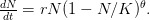
Bongaarts and Feeney (1998) introduced a correction to TFR that uses measures of birth order to remove the distortions.  Myrskylä et al. (2009) were able to apply the Bongaarts/Feeney correction to a sub-sample (41) of their 2005 data.  Of these 41 countries, they were able to calculate the tempo-adjusted TFR for 28 of the 37 countries with an HDI of 0.85 or greater in 2005. The countries with adjusted TFRs are plotted in black in their online supplement figure S2, reproduced here with permission.

Myrskyla_etal-figS2As one can easily see, the general trend of increasing TFR with HDI remains when the corrected TFRs are used.  This graphical result is confirmed by a formal statistical test: Following the coincident TFR minimum/HDI in the 0.86-0.9 window, the slope of the best-fit line through the scatter is positive.

Hugh notes repeatedly that Myrskylä et al. (2009) anticipated various criticisms that he levels.  For example, he writes "And you don’t have to rely on me for the suggestion that the Tfr is hardly the most desireable [sic] measure for what they want to do, since the authors themselves point this very fact out in the supplementary information." This seems like good honest social science research to me. I'm not entirely comfortable with the following paraphrasing, but here it goes.  We do science with the data we have, not the data we wish we had.  TFR is a widely available measure of fertility that allowed the authors to look at the relationship between fertility and human development over a large range of the HDI. Now, of course, having written a paper with the data that are available, we should endeavor to collect the data that we would ideally want.  The problem with demographic research though is that we are typically at the whim of the government and non-government (like the UN) organizations that collect official statistics.  It's not like we can go out and perform a controlled experiment with fixed treatments of human development and observe the resulting fertility patterns. So this paper seems like a good-faith attempt to uncover a pattern between human development and fertility.  When Hugh writes "the only thing which surprises me is that nobody else who has reviewed the research seems to have twigged the implications of this" (i.e., the use of  TFR as a measure of fertility), I think he is being rather unfair.  I don't know who reviewed this paper, but I'm certain that they had both a draft of the paper that eventually appeared in the print edition of Nature and the online Supplemental material in which Myrskylä and colleagues discuss the potential weaknesses of their measures and evaluate the robustness of their conclusions. That's what happens when you submit a paper and it undergoes peer review.  The pages of Nature are highly over-subscribed (as Nature is happy to tell you whenever it sends you a rejection letter).  Space is at a premium and the type of careful sensitivity analysis that would be de rigeur in the main text of a specialist journal  such as Demography, Population Studies, or Demographic Research, end up in the online supplement in Nature, Science, or PNAS.

On a related note, Hugh complains that the reference year in which the curvilinear relationship between TFR and HDI is shown is a bad year to pick:

Also, it should be remembered, as I mention, we need to think about base years. 2005 was the mid point of a massive and unsustainable asset and construction boom. I think there is little doubt that if we took 2010 or 2011, the results would be rather different.

The problem with this is that the year is currently 2009, so we can't use data from 2010 or 2011.  It seems entirely possible that the results would be different if we used 2011 data and I look forward to the paper in 2015 in which the Myrskylä hypothesis is re-evaluated using the latest demographic data.  This is sort of the nature of social science research.  There are very few Eureka! moments in social science.  As I note above, we can't typically do the critical experiment that allows us to test a scientific hypothesis.  Sometimes we can get clever with historical accidents (known in the biz as "natural experiments"). Sometimes we can use fancy statistical methods to approximate experimental control (such as the fixed effects estimation Myrskylä et al. use or the propensity score stratification used by Felton Earls and colleagues in their study of firearm exposure and violent behavior).  If we waited until we had the perfect data to test a social science hypothesis, there would never be any social science.  Perhaps things will indeed be different in 2011.  If so, we may even get lucky and by comparing why things were different in 2005 and 2011, gain new insight into the relationships between human development and fertility. Until then, I am going to credit Myrskylä and colleagues for opening a new chapter on our understanding of fertility transitions.

Oh, and I plan to cite the paper, as I'm sure many other demographers will too...

Reversal of Fertility Decline

In a terrific paper in the latest issue of Nature, Myrskylä and colleagues (including my sometime collaborator Hans-Peter Kohler) demonstrate that total fertility rate (TFR) -- which we typically think of as declining with economic development -- actually increases at very high levels of development.  One of the fundamental challenges of social science remains explaining the unprecedented decline in fertility witnessed in the twentieth century.  This fertility decline has gone hand-in-hand with economic development.  As Myrskylä et al. write, "The negative association of fertility with economic and social development has therefore become one of the most solidly established and generally accepted empirical regularities in the social sciences."

For those social scientists with an evolutionary bent, this observation has been particularly vexing since it appears to violate our expectations regarding resource-holding and reproductive success.  In a great many traditional societies, researchers have documented a positive relationship between wealth and reproductive success.  However, as soon as people are embedded within (and actually integrated with) the structures of a state-level society, this relationship apparently changes: rich people in states appear to have fewer children than poor people.  And as the overall level of wealth of a state increases, the aggregate pattern of fertility also decreases.  Now there are plenty of caveats here.  Many scholars have committed the ecological fallacy in attributing causal explanations at the individual level based on aggregate ("ecological") data. There is some evidence that the wealthy and well educated actually have marginally higher fertility in certain contexts, but the overwhelming weight of evidence shows that -- at least at the aggregate level -- increased wealth leads to decreased fertility. Until now.

The authors use the Human Development Index (HDI), a widely used measure of progress in human development.  The HDI combines three dimensions: (1) health, as measured by life expectancy at birth, (2) standard of living, as measured by the logarithm of per capita gross domestic product at purchasing power parity in US dollars, and (3) human capital as measured by adult literacy and the enrollment fraction in primary, secondary, and tertiary school.  HDI is now standardized so that it varies between zero and one.  This makes it easy to compare HDI across countries and through time.  The measure of fertility that Myrskylä and colleagues use is total fertility rate.  This is also probably the most commonly used measure of fertility.  It is the sum of a population's age-specific fertility rates across a woman's reproductive years, assuming that the woman survives this span.  It is a demographic fiction, but it is a useful fiction.

What Myrskylä et al. (2009) show (in their figure 1) is that TFR largely declines with HDI in 1975, as expected. The cool, unexpected finding that their paper reports is that in 2005, TFR declines with HDI to a point. When the HDI exceeds 0.9 though, fertility again increases. This plot is cross-sectional: it is a scatter plot of all countries' HDI-TFR pairs for a particular time period. One reason why we don't see this upward turn at the highest levels of human development in 1975 is that no countries had achieved this apparent threshold of HDI=0.9. Of course, from this plot we can't rule out the existence of some "period effect." That is, maybe there was just something different in society or the economy in 2005 compared to 1975.

back half template
Myrskylä et al. (2009) figure 1 (used with permission of the authors).

In figure 2, the authors plot longitudinal data for individual countries. They show that once HDI enters a window between 0.86-0.9 and TFR bottoms out, further increases in HDI lead to increases in TFR.

Myrskylä et al. (2009) figure 2 (used with permission of the authors)

This greatly increases our confidence that there is, in fact, a causal relationship between increased human development and fertility.  The really cool thing about this plot, however, is the exceptions to the general trend that it shows. In particular, Japan, South Korea, and Canada (and to a lesser extent Austria, Australia, and Switzerland) do not show this pattern.  For these countries, further increases in HDI are associated with further declines in TFR. A distinct possibility is that for some countries, increasing human welfare also leads to institutions that permit people (particularly women) to have children and be educationally and economically successful at the same time -- that is, not just people who were lucky enough to be born rich.  It's a shocking idea. The authors write:

[A]n improved understanding of how improved labour-market flexibility, social security and individual welfare, gender and economic equality, human capital and social/family policies can facilitate relatively high levels of fertility in advanced societies is needed. For instance, analyses on Europe show that nowadays a positive relationship is observed between fertility and indicators of innovation in family behaviour or female labour-force participation. Also, at advanced levels of development, governments might explicitly address fertility decline by implementing policies that improve gender equality or the compatibility between economic success, including labour force participation, and family life. Failure to answer to the challenges of development with institutions that facilitate work–family balance and gender equality might explain the exceptional pattern for rich eastern Asian countries that continue to be characterized by a negative HDI–fertility relationship.

These are important problems and this is a fundamental contribution to our understanding of the relationships between economic development, human welfare, and reproductive behavior.

Bill O'Reilly Discovers New Demographic Principle

So, either Bill O'Reilly is either on to something profound or he simply doesn't understand averages.  Methinks it's the latter. It's actually a pretty common problem -- people not understanding life expectancy -- it's just that O'Reilly boffs it in such spectacular form! Mathematical expectation is a fancy term for taking an average. You know, sum up the values and divide by the number of cases? In the case of life expectancy, the thing that we're averaging over is the number of years lived by members of a well-defined population. Mechanistically, when we calculate the life expectancy at age x we take all the person-years still to be lived by this group of people and divide by the number who started at age x.  The United States has ten times the number of deaths from accidents, etc. as Canada, but it also has ten times the number of people starting at age zero. Oops. I also love the fact that he seems to be attributing the differences in life expectancy between Canada and the United States not to differences in our health care systems but in societal pathologies like more accidents and crime in the United States!

Why Use R?

An anthropologist colleague who did a post-doc in a population center has been trying to get a group of people at his university together to think about population issues.  This is something I'm all for and am happy to help in whatever little way I can to facilitate especially anthropologists developing their expertise in demography.  One of the activities they have planned for this population interest group is a workshop on the R statistical programming language. The other day he wrote me with the following very reasonable question that has been put to him by several of the people in his group: Sure R is free but other than that why should someone bother to learn new software when there is perfectly acceptable commercial software out there?  This question is particularly relevant when one works for an institution like a university where there are typically site licenses and other mechanisms for subsidizing the expense of commercial software (which can be substantial).  What follows is, more or less, what I said to him.

I should start out by saying that there is a lot to be said for free. I pay several hundred dollars a year for commercial software that I don't actually use that often. Now, when I need it, it's certainly nice to know it's there but if I didn't have a research account paying for this software, I might let at least one or two of these licenses slide.  I very occasionally use Stata because the R package that does generalized linear mixed models has had a bug in the routine that fits logistic mixed models and this is something that Stata does quite well. So I regularly get mailings about updates and I am always just blown away at the expense involved in maintaining the most current version of this software, particularly when you used the intercooled version.  It's relatively frequently updated (a good thing) but these updates are expensive (a bad thing for people without generous institutional subsidies). So, let me just start by saying that free is good.

This actually brings up a bit of a pet peeve of mine regarding training in US population centers.  We have these generous programs to train population scientists and policy-makers from the poor countries of the world.  We bring them into our American universities and train them in demographic and statistical methods on machines run by proprietary (and expensive!) operating systems and using extremely expensive proprietary software.  These future leaders will graduate and go back home to Africa, Asia, eastern Europe, or Latin America. There, they probably won't have access to computers with the latest hardware running the most recent software.  Most of their institutions can't afford expensive site licenses to the software that was on every lab machine back at Princeton or UCLA or Michigan or [fill in your school's name here]. This makes it all the more challenging to do the work that they were trained to do and leaves them just that much more behind scholars in advanced industrial nations.  If our population centers had labs with computers running Linux, taught statistics and numerical methods using R, and had students write LaTeX papers, lecture slides, and meeting posters using, say, Emacs rather than some bloated word-processor whose menu structure seems to change every release, then I think we would be doing a real service to the future population leaders of the developing world. But let's return to the question at hand, other than the fact that it's free -- which isn't such an issue for someone with a funded lab at an American University -- why should anyone take the trouble to learn R? I can think of seven reasons off the top of my head.

(1) R is what is used by the majority of academic statisticians.  This is where new developments are going to be implemented and, perhaps more importantly, when you seek help from a statistician or collaborate with one, you are in a much better position to benefit from the interaction if you share a common language.

(2) R is effectively platform independent.  If you live in an all-windows environment, this may not be such a big deal but for those of us who use Linux/Mac and work with people who use windows, it's a tremendous advantage.

(3) R has unrivaled help resources.  There is absolutely nothing like it.  First, the single best statistics book ever is written for R (Venables & Ripley, Modern Applied Statistics in S -- remember R is a dialect of S).  Second, there are all the many online help resources both from r-project.org and from many specific lists and interest groups. Third, there are proliferating publications of excellent quality. For example, there is the new Use R series. The quantity and quality of help resources is not even close to matched by any other statistics application.  Part of the nature of R -- community constructed, free software -- means that the developers and power users are going to be more willing to provide help through lists, etc. than someone in a commercial software company. The quality and quantity of help for R is particularly relevant when one is trying to teach oneself a new technique of statistical method.

(4) R makes the best graphics. Full stop. I use R, Matlab, and Mathematica.  The latter two applications have a well-deserved reputation for making great graphics, but I think that R is best.  I quite regularly will do a calculation in Matlab and export the results to R to make the figure.  The level of fine control, the intuitiveness of the command syntax (cf. Matlab!), and the general quality of drivers, etc. make R the hands-down best.  And let's face it, cool graphics sell papers to reviewers, editors, etc.

(5) The command-line interface -- perhaps counterintuitively -- is much, much better for teaching.  You can post your code exactly and students can reproduce your work exactly.  Learning then comes from tinkering. Now, both Stata and SAS allow for doing everything from the command line with scripts like do-files.  But how many people really do that?  And SPSS...

(6) R is more than a statistics application.  It is a full programming language. It is designed to seamlessly incorporate compiled code (like C or Fortran) which gives you all the benefits of a interactive language while allowing you to capitalize on the speed of compiled code.

(7) The online distribution system beats anything out there.

Oh, and let's face it, all the cool kids use it...

New Publication: Chimpanzee "AIDS"

keele_etal2009-first-pageA long-anticipated paper (by me anyway!) has finally been published in this week's issue of Nature.  In this paper, we show that wild chimpanzees living in the Gombe National Park in western Tanzania on the shores of Lake Tanganyika appear to die from AIDS-like illness when infected with the Simian Immunodeficiency Virus (SIV).  Many African primates harbor their own species-specific strain of SIV and chimpanzees are no exception.  The host species for a particular SIV strain is indicated by a three letter abbreviation (all in lower-case) following the all-caps SIV. So, for chimpanzees, the strain is called SIVcpz. It turns out that there are two distinct HIVs, known as HIV-1 and HIV-2. HIV-1 is the virus that causes the majority of the world's deaths.  It is what we call the "pandemic strain." HIV-2 is less pathogenic and has a distinct geographic focus in West Africa.  The HIVs and the various SIVs belong to a larger group of viruses that infect a wide range of mammals known as the lentiviruses (lenti- meaning slow, referring to the slow time course of the pathology typically caused by these viruses). Collectively, we call the SIVs and HIVs "primate lentiviruses."  Both HIV-1 and HIV-2 have well-documented origins in nonhuman primate reservoirs.  HIV-2 is most closely related to SIVsmm, a virus that infects sooty mangebeys (a type of West-African monkey).  HIV-1, on the other hand, is most closely related to SIVcpz, the virus that infects central and east African chimpanzees.  We believe that both HIV-1 and HIV-2 entered humans hosts when hunters were contaminated with the blood of infected monkeys (HIV-2) or chimpanzees (HIV-1). Note that this means that our terminology for the primate lentiviruses is polyphyletic.  SIVsmm and HIV-2 are sister species, while SIVcpz and HIV-1 are sister species.  Yet we call all the viruses that infect nonhuman primates simian and all the viruses that infect humans human immunodeficiency viruses.  It seems to me the best way to fix this would be to call the viruses that infect humans SIVhum1 and SIVhum2.  Of course, that will never happen, but I do think that it's important to clarify the evolutionary history of these viruses.

The conventional wisdom regarding primate lentiviruses is that, with the exception of HIV, they are not pathogenic in their natural host.  The reasoning for why HIV causes the devastating pathology that characterizes AIDS goes that HIV-1 is a relatively new infection of humans, having just spilled over into the human population recently.  Pathogens that have recently crossed species boundaries are frequently highly pathogenic because neither the new host nor the pathogen has a history of coevolution with its new partner.  While it is a pernicious myth (that just won't seem to die) that pathogens necessarily evolve toward a benign state, it is true that they frequently evolve a more intermediate level of virulence from their initial spillover virulence.  There are a number of problems with the idea that HIV causes AIDS because it is poorly adapted to human physiology.

The first of these is that HIV-1 is not that recent an infection of humans.  Sure, we didn't notice it until 1983 but careful molecular evolutionary analysis by Bette Korber of the Santa Fe Institute and my collaborator Beatrice Hahn and her group at the University of Alabama Birmingham puts the most likely date for the emergence of HIV-1 in humans to be 1931.  That means that HIV-1 was being transmitted from human-to-human for over fifty years before it was ever noticed by western science. Fifty years, while certainly brief in evolutionary terms, is still long enough to lead to some reduction in virulence or host evolution.

The real nail in the coffin, however, is our new result.  Specifically, we show that SIVcpz causes AIDS-like pathology in the Gombe chimpanzees. This result is surprising because (1) given it's pathogenicity, one would expect someone to have noticed it before, and (2) chimpanzees infected in captivity do not show obvious AIDS-like illness. I have been collaborating with Anne Pusey, Mike Wilson and their colleagues at the University of Minnesota's Jane Goodall Institute Center for Primate Studies on the the analysis of the demography of the Gombe chimps for a number of years now. Anne and Mike have, in turn, been collaborating with Beatrice Hahn with her project on monitoring natural SIV infection in wild chimpanzees across Africa. Given my background in HIV epidemiology and statistics, it was only natural that we all join forces to look at the demographic implications of SIV infection among the Gombe chimps.  Jane Goodall famously started chimpanzee research at Gombe in 1960 and since 1964, researchers at Gombe have collected detailed demographic information, documenting all births, deaths, and migration events in the central community and eventually expanding to the peripheral ones in later years. As a result, we have an unmatched level of demographic detail (not to mention behavioral and ecological information) against which to assess the impact of SIV infection.  Using statistical methods known collectively as event-history analysis, we were able to show that the hazard ratio between SIV-infected and SIV-negative chimps is on the order of 10-16.  This essentially means that SIV+ chimps have mortality rates that are 10-16 times higher than uninfected chimps.  The analysis controls for the clear potentially confounding effects of age and sex on overall mortality. The reason why no one ever noticed this heightened mortality rate is really because no one has ever looked for it. Even when a mortality rate is 10 times higher for some segment of a population, when that segment is small and when mortality rates quite low (chimps who survive infancy can live in excess of 40 years) it can be hard to detect even a seemingly large difference.  This is why we do science: because things that seem obvious once we know they are there can be remarkably subtle when we don't know they're there.  Science gives us the framework and the tools for studying nature's subtleties.

This project was absurdly interdisciplinary.  The paper has 22 co-authors, each contributing his or her own particular analytical expertise or providing access to crucial data necessary for the larger narrative.  There are papers in the literature in which people are made co-authors for pretty thin contributions.  This paper has none of that.  It was an extremely complicated story to tell and it really required the collaboration of this large team. Such work is not easy to manage and it's not at all easy to do well.  I think that Beatrice should be commended for orchestrating all the various major contributions, keeping us in line and on schedule (more or less). It's really gratifying to see the excellent blog piece by Carl Zimmer in which he notes the virtues -- and the difficulty -- of combining various scientific styles in pursuit of an important question. The title of Carl's piece is "AIDS and the Virtues of Slow-Cooked Science." In addition, there is a nice companion piece in this week's Nature written by Robin Weiss and Jonathan Heeney.  They too note the strength of the interdisciplinary approach to this problem.

The paper isn't even officially published until tomorrow and it has already been covered on Carl Zimmer's blog for Discover Magazine, The New ScientistThe GuardianThe ScientistThe New York Times and MSNBC. Wow.  Weiss & Heeney note a number of questions that are raised by our analysis.  Specifically, they ask "why was the progression to AIDS-like illness not more apparent in chimpanzees in captivity?" My co-author Paul Sharp notes "We need to know much more about whether there are any genetic differences among the chimpanzees, or differences in co-infections with other viruses, bacteria or parasites, which influence whether or not SIV infection leads to illness or death. This presents a unique opportunity to compare and contrast the disease-causing mechanisms of two closely related viruses in two closely related hosts."  Then, of course, there are the conservation questions that this paper raises.  Chimpanzees in the wild have birth rates that are very nearly balanced out by their death rates.  This difference, called the intrinsic rate of increase, largely determines the probability of extinction of a small population.  When the rate of increase of a population is negative, it is certain to go extinct (assuming the rate remains negative).  However, even if the intrinsic rate of increase is greater than zero, the randomness that besets small populations still means that a population can go extinct.  So, because their average birth and death rates are so close, individual chimp populations are certainly in potential jeopardy of going extinct, and Gombe is no exception to this rule. Now we add to a population something that increases mortality rates 10-16 times.  This is bound to have negative consequences for the persistence of affected chimp populations.  This is a topic that we are exploring even as I write...

Happy Birthday Demography!

I received a note from Rich Lawler this morning, who passed along a note he received from Hal Caswell, who passed along a note he, in turn, received from someone at the Max Planck Institute for Demographic Research (where my friend Josh Goldstein is Director).  In this note, I was reminded that today is the 348th birthday of demography! You see, on this date (27 February) in 1661, John Graunt read his paper, "Natural and Political Observations Mentioned in a Following Index, and Made Upon the Bills of Mortality," to the Royal Society of London.  At the time of his writing, London had begun to keep track of the number of burials and christenings taking place within its jurisdiction.  In good empiricist Baroque British style, Graunt managed to extract an amazing amount of information from these data.  And this is really what demographers do to this day: we count things like births, deaths, and marriages and make inferences about the way the world works from these simple counts.

In this essay, Graunt mused about why one might want to do things like count deaths and births:

There seems to be good reason why the Magistrate should himself take notice of the numbers of burials and christenings, viz., to see whether the City increase or decrease in people; whether in increase proportionately with the rest of the Nation; whether it be grown big enough, or too big, etc.

Good practical reasons why one might want to count births and deaths. Perhaps the most notable thing that Graunt did in his essay is to construct the first life table, that mainstay of demographic analysis. Actually, at least one of life table actually existed in ancient Rome (attributed to Ulpian, 3rd century C.E.), but Graunt was certainly the first to write about a life table. He reasons:

Whereas we have found that of 100 quick conceptions about 36 of them die before they be six years old, and that perhaps but one surviveth 76, we, having seven decades between six and 76, we sought six mean proportional numbers between 64, the remainder living at six years, and the one which survives 76, and find that the numbers following are practically near enough to the truth; for men do not die in exact proportions, nor in fractions: from when arises this Table following:

Viz of 100 there dies within the first six years 36

The next ten years, or decade                          24

The second decade                                           15

The third decade                                                9

The fourth                                                          6 

The next                                                             4

The next                                                             3

The next                                                             2

The next                                                             1


With his radix set to 100, this means that "of the said 100 conceived there remains alive at six years end 64,

At sixteen years end  40

At twenty-six             25

At thirty-six               16

At forty-six                10

At fifty-six                   6

At sixty-six                 3

At seventy-six             1

At eighty                      0"

Fortunately, as demographic methodology has improved, I think the idea behind a life table has gotten easier to understand too.  He has a point though.  Men don't die in fractions.  This leads to a phenomenon that can be an issue in small populations known as demographic stochasticity. 

I particularly love the causes of death that Graunt enumerates.  Here are the "notorious diseases": Apoplexy (1,306), Cut of the Stone (38), Falling Sickness (74), Dead in the streets (243), Gowt (134), Head-Ache (51), Jaundice (998), Lethargy (67), Leprosy (6), Lunatick (158), Overlaid, and Starved (529), Palsy (423), Rupture (201), Stone and Strangury (863), Sciatica (5), Sodainly (454).

And here are the "casualties": Bleeding (69), Burt and Scalded (125), Drowned (829), Excessive drinking (2), Frighted (22), Grief (279), Hanged themselves (222), Killed by several accidents (1,021), Murdered (86), Poisoned (14), Smothered (26), Shot (7), Starved (51), Vomiting (136).

Just in case you were still harboring illusions that 17th century London was not a violent place...

Durkheim is typically credited with discovering structure in society.  Seems to me like John Graunt might have a claim to that 200 years before him.  Surely, there is an implied regularity to the means by which death is meted out in Graunt's primitive life table.  Much of Graunt's essay can be found here. The full text can be found in the Journal of the Institute of Actuaries, 1964, volume 90.

Further Adventures in Publishing

I finally received the pdf version of my recently published paper with a 2006 publication date.  My grad student, Brodie Ferguson, and I used demographic data from the Colombia censuses of 1973, 1985, 1993, and 2002 to calculate the magnitude of the marriage squeeze felt by women in Colombia.  The protracted civil conflict in Colombia means that there has been a burden of excess young male mortality in that country for at least 30 years (the measurement of which is the subject of a paper soon to be submitted).  This excess male mortality means that there are far more women entering the marriage market than there are men, putting the squeeze on women (i.e., making it more difficult for them to marry).  Our results show that in the most violent Colombian departments at the height of the violence (1993), the marital sex ratio was as low at 0.67.  This means for every 100 men entering the marriage market, there were 150 women.  This is a truly stunning number.  We discuss some of the potential societal consequences of these incredibly unbalanced sex ratios.  Two very important phenomena that we think are linked to these extraordinary sex ratios are: (1) the high rates of consensual unions (i.e., non-married couples "living together") in Colombia and (2) the pattern of female-biased rural-urban migration.

The citation to the paper (even though it came out in 2008) is:

Jones, J. H., and B. D. Ferguson. 2006. The Marriage Squeeze in Colombia, 1973-2005: The Role of Excess Male Death. Social Biology. 53 (3-4):140-151.

Plotting Recruitment Curves

I was asked how I plotted the recruitment curve from my last post. It's pretty easy to do in R.

[r]
Dn <- expression(r * (1 - N/K) * N) r <- 0.004 K <- 10^10 N <- seq(0,10^10,by=10^7) png(file="recruitment.png") ## sends output to .png file plot(N,eval(Dn),type="l", xlab="Human Population", ylab="Recruitment") dev.off() [/r]

Now we can generalize to the generalized theta logistic model where

 \frac{dN}{dt} = rN(1-N/K)^{\theta}.

This model changes the shape of the density dependence when \theta<1 the density dependence is felt only at higher densities, whereas when \theta>1 the density dependence kicks in at low population size.

Consider our problem of what the optimal harvest size of humans by Kanamits consumers would be if human population size was actually regulated according to the theta-logistic model. First, we assume that \theta<1.

[r]
Dn.gen <- expression((r * (1 - N/K))^theta * N) theta <- 0.1 png(file="recruitment-thless1.png") plot(N,eval(Dn.gen),type="l", xlab="Human Population", ylab="Recruitment") title("theta=0.1") dev.off() [/r]

Now, we assume that \theta>1.

[r]
theta <- 10 png(file="recruitment-thgr1.png") plot(N,eval(Dn.gen),type="l", xlab="Human Population", ylab="Recruitment") title("theta=10") dev.off() [/r]

I sent the output to a portable network graphics (png) device because I wanted to include the figures with this post. Normally, in interactive work, you would send this to the default on-screen device (e.g., x11 or Quartz). When making a figure for publication or to include with a LaTeX document, one would send the output to a pdf device.

From this example, we can see that the shape of the density dependence can pretty drastically change the MSY, at least in the case where the discount rate is zero. When \theta=10, we can see that the Kanamits would only be able to sustainably harvest on the order of a billion people, whereas if \theta=0.1, they could take nearly 9 billion and still have a viable population. I'm guessing that the former is closer to the truth than the latter, but let's hope that the answer remains in the realm of absurdist speculation where it belongs.